Both iscream and Rsamtools can be used to query records from tabixed BED files in R. Here we compare their usability and performance using the methscan dataset.
This vignette uses mouse WGBS data from methscan as in the Plotting TSS profiles tutorial and mouse promoter regions. Running it requires downloading 18MB of BED files and tabix indices from this Zenodo record: https://zenodo.org/records/18089082
library("BiocFileCache") |> suppressPackageStartupMessages()
cachedir <- BiocFileCache()
methscan_zip_path <- bfcrpath(cachedir, "https://zenodo.org/records/18089082/files/methscan_data.zip")
methscan_unzip <- file.path(tempdir(), "methscan")
unzip(methscan_zip_path, exdir = methscan_unzip)
methscan_dir <- file.path(methscan_unzip, "scbs_tutorial_data")
iscream normally uses htslib to query BED files and store the data in
memory. However, iscream’s tabix() function can use the
tabix executable to make tabix queries because the shell program’s
stream-to-file approach is faster than allocating and storing strings in
memory. By default, the "tabix.method" option is set to
“shell” and iscream’s tabix() will look for the tabix
executable, falling back to using htslib only if it’s not found. Here,
the "tabix.method" option is set to “htslib” to make fair
comparisons between Rsamtools and iscream since scanTabix
does not use the executable, but stores the strings in memory.
## iscream using 1 thread by default but parallelly::availableCores() detects 16 possibly available threads. See `?set_threads` for information on multithreading before trying to use more.Using scanTabix requires the input regions to be
GRanges. iscream::tabix accepts strings, data
frames and GRanges.
library(data.table)
library(GenomicRanges) |> suppressPackageStartupMessages()
library(Rsamtools) |> suppressPackageStartupMessages()
library(microbenchmark)
library(pbapply)
library(ggplot2)
methscan_files <- list.files(
  methscan_dir,
  full.names = T,
  pattern = "*.cov.gz$"
)
mouse_promoters <- fread(file.path(methscan_dir, "mouse_promoters.bed"), col.names = c("chr", "start", "end"))
mouse_promoters.gr <- GRanges(mouse_promoters)
One file
tabix_raw() and scanTabix produce a list of
unparsed or raw strings. The result of both are identical.
bench_1_raw <- microbenchmark(
  `rsamtools 1 file raw` = rq <- scanTabix(methscan_files[1], param = mouse_promoters.gr),
  `iscream 1 file raw` = iq <- tabix_raw(methscan_files[1], mouse_promoters),
  times = 3
)
bench_1_raw
## Unit: milliseconds
## expr min lq mean median uq
## rsamtools 1 file raw 2760.55888 2765.35353 2769.3114 2770.14819 2773.68760
## iscream 1 file raw 79.47893 80.34265 84.7329 81.20637 87.35989
## max neval
## 2777.22701 3
## 93.51341 3
autoplot(bench_1_raw)## Warning: `aes_string()` was deprecated in ggplot2 3.0.0.
## ℹ Please use tidy evaluation idioms with `aes()`.
## ℹ See also `vignette("ggplot2-in-packages")` for more information.
## ℹ The deprecated feature was likely used in the microbenchmark package.
## Please report the issue at <https://github.com/joshuaulrich/microbenchmark/issues/>.
## This warning is displayed once every 8 hours.
## Call `lifecycle::last_lifecycle_warnings()` to see where this warning was generated.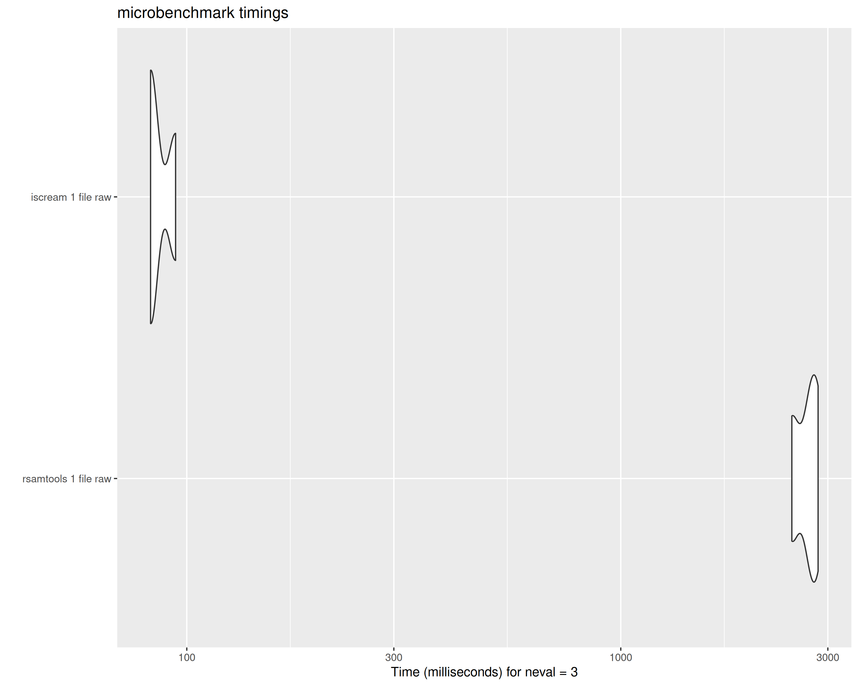
tabix vs scanTabix raw string output on 1 file
iq[1:5]## $`1:3669498-3673498`
## character(0)
##
## $`1:4407241-4411241`
## character(0)
##
## $`1:4494413-4498413`
## character(0)
##
## $`1:4783739-4787739`
## [1] "1\t4785488\t4785488\t0.000000\t0\t2"
## [2] "1\t4785513\t4785513\t0.000000\t0\t2"
## [3] "1\t4785522\t4785522\t0.000000\t0\t2"
## [4] "1\t4785533\t4785533\t0.000000\t0\t2"
## [5] "1\t4786780\t4786780\t100.000000\t1\t0"
## [6] "1\t4786886\t4786886\t100.000000\t1\t0"
## [7] "1\t4786958\t4786958\t100.000000\t1\t0"
##
## $`1:4805823-4809823`
## [1] "1\t4806176\t4806176\t100.000000\t1\t0"
## [2] "1\t4806221\t4806221\t100.000000\t1\t0"
## [3] "1\t4807572\t4807572\t0.000000\t0\t1"
## [4] "1\t4807669\t4807669\t0.000000\t0\t2"
## [5] "1\t4807682\t4807682\t0.000000\t0\t2"
## [6] "1\t4807872\t4807872\t0.000000\t0\t1"
## [7] "1\t4807890\t4807890\t0.000000\t0\t1"
## [8] "1\t4807940\t4807940\t0.000000\t0\t1"
## [9] "1\t4807950\t4807950\t0.000000\t0\t1"
all.equal(iq, rq)## [1] TRUEMultiple files
tabix() can also take multiple files in the same call.
It returns the raw strings, but each input file is a list of it’s own.
scanTabix() does not support this.
bench_30_raw <- microbenchmark(
  `iscream 30 files raw` = iq <- tabix_raw(methscan_files, mouse_promoters),
  times = 3
)
bench_30_raw
## Unit: seconds
## expr min lq mean median uq max
## iscream 30 files raw 1.346655 1.559583 1.859358 1.772512 2.115709 2.458907
## neval
## 3
names(iq)## [1] "cell_01" "cell_02" "cell_03" "cell_04" "cell_05" "cell_06" "cell_07"
## [8] "cell_08" "cell_09" "cell_10" "cell_11" "cell_12" "cell_13" "cell_14"
## [15] "cell_15" "cell_16" "cell_17" "cell_18" "cell_19" "cell_20" "cell_21"
## [22] "cell_22" "cell_23" "cell_24" "cell_25" "cell_26" "cell_27" "cell_28"
## [29] "cell_29" "cell_30"
iq[["cell_01"]][1:5]## $`1:3669498-3673498`
## character(0)
##
## $`1:4407241-4411241`
## character(0)
##
## $`1:4494413-4498413`
## character(0)
##
## $`1:4783739-4787739`
## [1] "1\t4785488\t4785488\t0.000000\t0\t2"
## [2] "1\t4785513\t4785513\t0.000000\t0\t2"
## [3] "1\t4785522\t4785522\t0.000000\t0\t2"
## [4] "1\t4785533\t4785533\t0.000000\t0\t2"
## [5] "1\t4786780\t4786780\t100.000000\t1\t0"
## [6] "1\t4786886\t4786886\t100.000000\t1\t0"
## [7] "1\t4786958\t4786958\t100.000000\t1\t0"
##
## $`1:4805823-4809823`
## [1] "1\t4806176\t4806176\t100.000000\t1\t0"
## [2] "1\t4806221\t4806221\t100.000000\t1\t0"
## [3] "1\t4807572\t4807572\t0.000000\t0\t1"
## [4] "1\t4807669\t4807669\t0.000000\t0\t2"
## [5] "1\t4807682\t4807682\t0.000000\t0\t2"
## [6] "1\t4807872\t4807872\t0.000000\t0\t1"
## [7] "1\t4807890\t4807890\t0.000000\t0\t1"
## [8] "1\t4807940\t4807940\t0.000000\t0\t1"
## [9] "1\t4807950\t4807950\t0.000000\t0\t1"## Error in h(simpleError(msg, call)): error in evaluating the argument 'file' in selecting a method for function 'scanTabix': 'file' must be length 1Parsing records into a data frame
A parsed data frame is more useful than a list of raw strings - use
tabix() instead of tabix_raw(). For
scanTabix, this custom function parses the list of strings
to make a similar data frame:
rtbx <- function(bed) {
  q <- scanTabix(bed, param = GRanges(mouse_promoters)) |>
    lapply(strsplit, split = "\t") |>
    Filter(function(i) length(i) != 0, x = _) |>
    unlist(recursive = FALSE) |>
    do.call(rbind, args = _) |>
    as.data.table() |>
    setnames(c("chr", "start", "end", paste0("V", 1:3)))
  q
}

bench_1_df <- microbenchmark(
  `rsamtools 1 file data frame` = rq <- rtbx(methscan_files[1]),
  `iscream 1 file data frame` = iq <- tabix(methscan_files[1], mouse_promoters),
  times = 3
)
rq
## chr start end V1 V2 V3
## <char> <char> <char> <char> <char> <char>
## 1: 1 4785488 4785488 0.000000 0 2
## 2: 1 4785513 4785513 0.000000 0 2
## 3: 1 4785522 4785522 0.000000 0 2
## 4: 1 4785533 4785533 0.000000 0 2
## 5: 1 4786780 4786780 100.000000 1 0
## ---
## 79900: X 168673566 168673566 0.000000 0 1
## 79901: X 168673577 168673577 0.000000 0 1
## 79902: X 168674670 168674670 0.000000 0 1
## 79903: X 168675047 168675047 0.000000 0 1
## 79904: X 169318831 169318831 100.000000 1 0
iq## chr start end V1 V2 V3
## <char> <int> <int> <num> <int> <int>
## 1: 1 4785488 4785488 0 0 2
## 2: 1 4785513 4785513 0 0 2
## 3: 1 4785522 4785522 0 0 2
## 4: 1 4785533 4785533 0 0 2
## 5: 1 4786780 4786780 100 1 0
## ---
## 79900: X 168673566 168673566 0 0 1
## 79901: X 168673577 168673577 0 0 1
## 79902: X 168674670 168674670 0 0 1
## 79903: X 168675047 168675047 0 0 1
## 79904: X 169318831 169318831 100 1 0
all.equal(iq, rq, check.attributes = F)## [1] "Datasets have different column modes. First 3: start(numeric!=character) end(numeric!=character) V1(numeric!=character)"The column types are different but the data is identical.
bench_1_df## Unit: milliseconds
## expr min lq mean median uq
## rsamtools 1 file data frame 2169.4535 2229.954 2641.8171 2290.4544 2877.9989
## iscream 1 file data frame 132.9694 134.259 141.7589 135.5487 146.1537
## max neval
## 3465.5434 3
## 156.7588 3
autoplot(bench_1_df)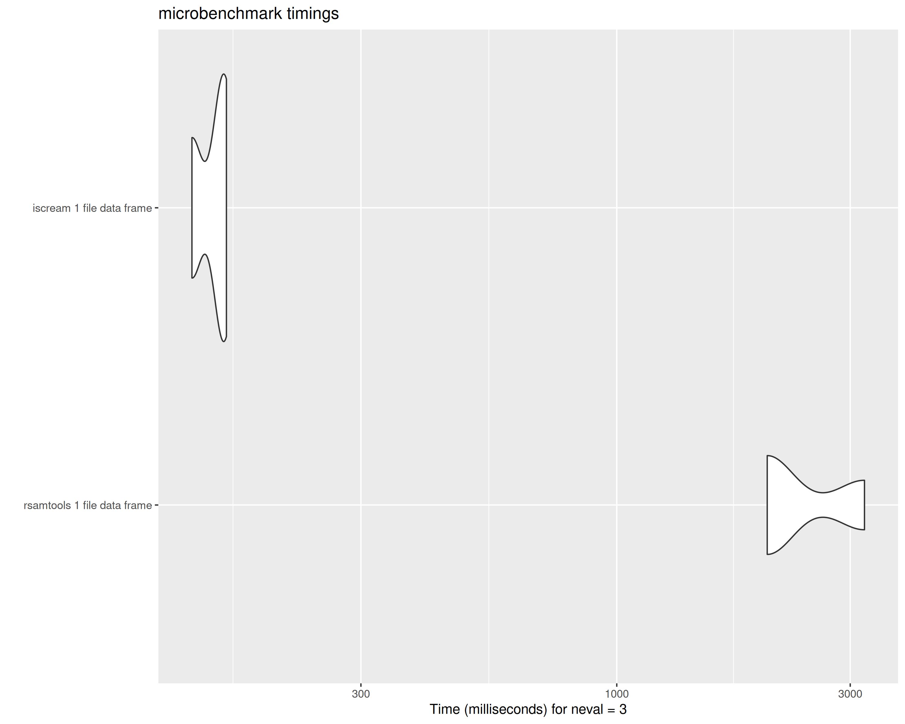
tabix vs scanTabix parsed data frame from 1 file
Multiple files as data frame
We can try to query multiple BED files using Rsamtools with this function that uses 8 cores like iscream does:
partbx <- function(bedfiles) {
  pblapply(
    methscan_files,
    function(bed) {
      query <- rtbx(bed)[, file := tools::file_path_sans_ext(basename(bed), compression = TRUE)][]
      setnames(query, c("chr", "start", "end", "beta", "M", "U", "file"))
      query
    },
    cl = 8
  ) |>
    rbindlist()
}

bench_30_df <- microbenchmark(
  `rsamtools 30 file data frame` = rq <- partbx(methscan_files),
  `iscream 30 file data frame` = iq <- tabix(methscan_files, mouse_promoters, col.names = c("beta", "M", "U")),
  times = 3
)
bench_30_df
## Unit: seconds
## expr min lq mean median uq
## rsamtools 30 file data frame 24.823254 26.949417 28.924390 29.07558 30.974959
## iscream 30 file data frame 1.074239 1.389884 1.660032 1.70553 1.952928
## max neval
## 32.874338 3
## 2.200326 3
autoplot(bench_30_df)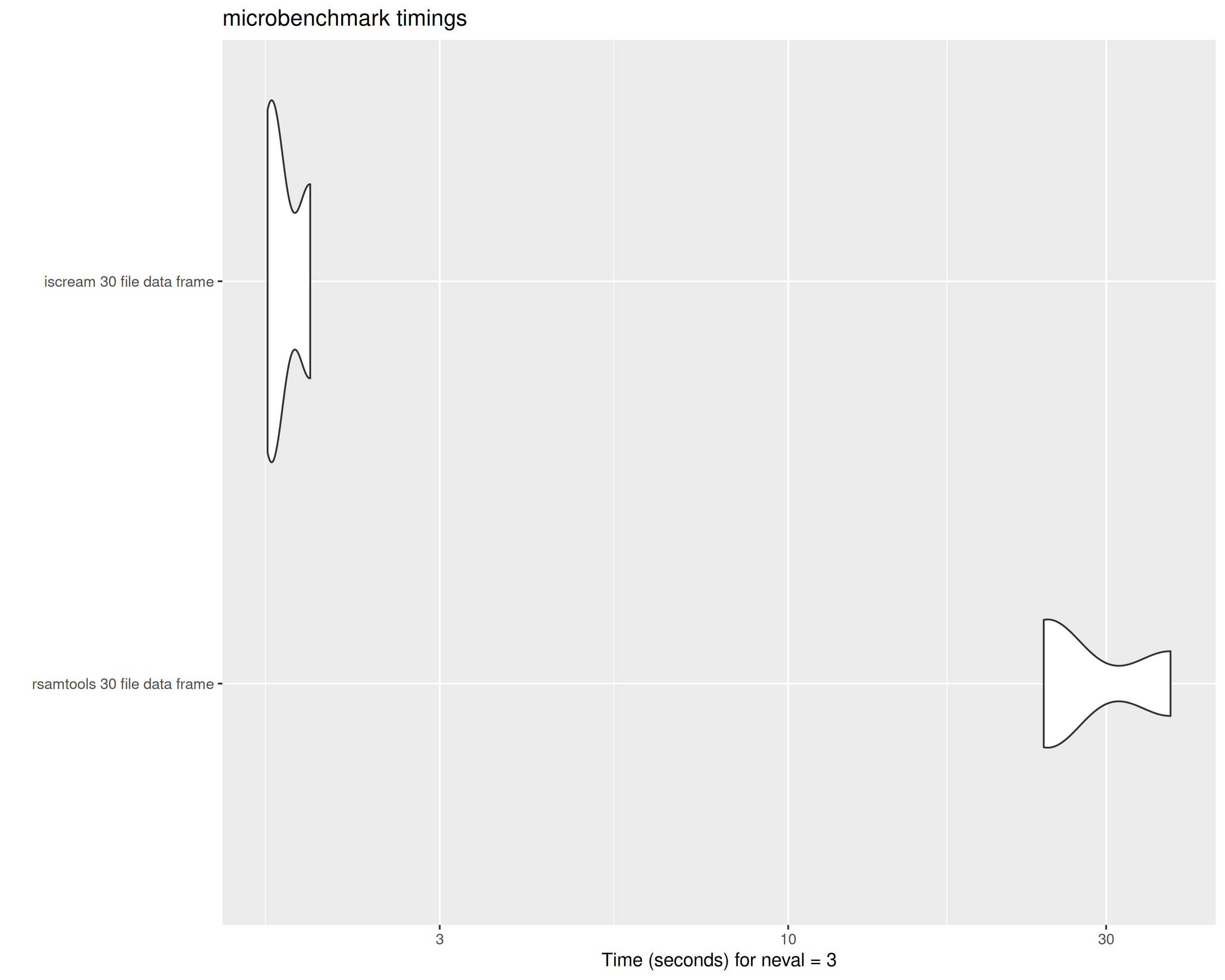
tabix vs scanTabix parsed data frame from 30 files
All benchmarks
bench_all <- rbind(bench_1_raw, bench_30_raw, bench_1_df, bench_30_raw, bench_30_df)

bench.dt <- as.data.table(bench_all)[, .(
  time       = time / 1000000,
  package    = fifelse(grepl("iscream", expr), "iscream", "rsamtools"),
  files      = fifelse(grepl("1", expr), 1, 30),
  data.frame = fifelse(grepl("raw", expr), FALSE, TRUE)
)][,
  `data structure` := fifelse(data.frame, "data.frame", "raw-strings")
]
Runtime
ggplot(bench.dt, aes(x = as.factor(files), y = time / 1000, color = as.factor(package))) +
  geom_boxplot(position = position_dodge(preserve = "single")) +
  scale_color_discrete(name = "Package") +
  scale_y_continuous(limits = c(0, 35), breaks = scales::extended_breaks(10)) +
  facet_wrap(~ `data structure`, labeller = "label_both") +
  labs(x = "File count", y = "Runtime (seconds)") +
  theme_bw()
## Warning: Removed 1 row containing non-finite outside the scale range
## (`stat_boxplot()`).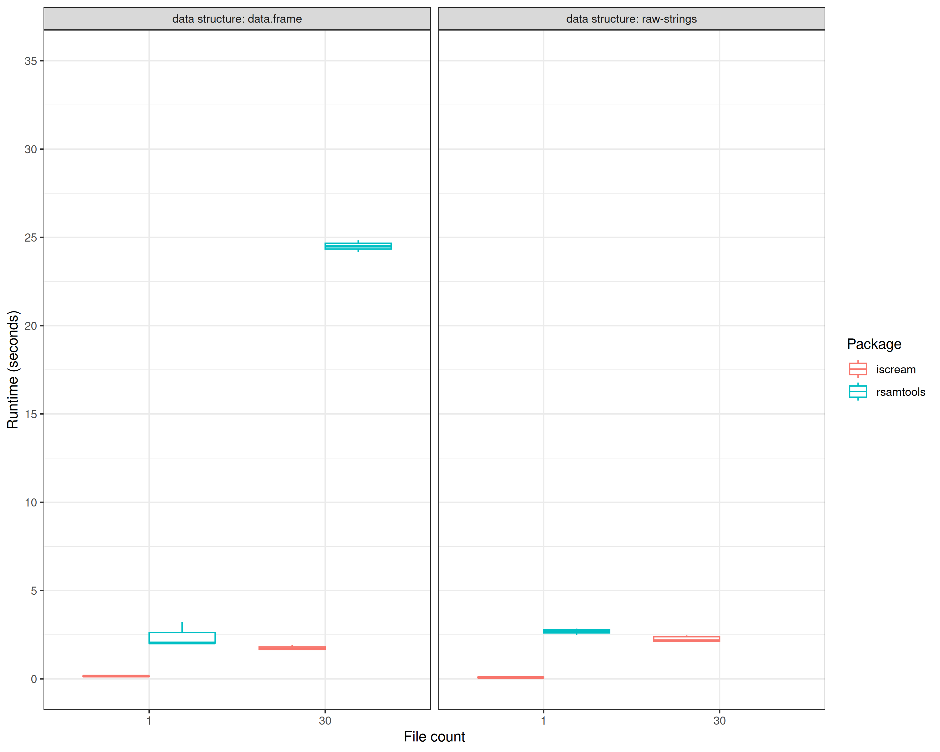
Comparing all benchmarked iscream and Rsamtools querying runtimes
Session info
## R version 4.5.1 (2025-06-13)
## Platform: x86_64-pc-linux-gnu
## Running under: Ubuntu 24.04.3 LTS
##
## Matrix products: default
## BLAS/LAPACK: /nix/store/g5b7qnbhjmiac5q4jb5yvahy6pysd88g-blas-3/lib/libblas.so.3;  LAPACK version 3.12.0
##
## locale:
##  [1] LC_CTYPE=en_US.UTF-8       LC_NUMERIC=C
##  [3] LC_TIME=en_US.UTF-8        LC_COLLATE=en_US.UTF-8
##  [5] LC_MONETARY=en_US.UTF-8    LC_MESSAGES=en_US.UTF-8
##  [7] LC_PAPER=en_US.UTF-8       LC_NAME=C
##  [9] LC_ADDRESS=C               LC_TELEPHONE=C
## [11] LC_MEASUREMENT=en_US.UTF-8 LC_IDENTIFICATION=C
##
## time zone: America/Detroit
## tzcode source: system (glibc)
##
## attached base packages:
## [1] stats4    stats     graphics  grDevices utils     datasets  methods
## [8] base
##
## other attached packages:
##  [1] ggplot2_4.0.0        pbapply_1.7-4        microbenchmark_1.5.0
##  [4] Rsamtools_2.25.3     Biostrings_2.77.2    XVector_0.49.1
##  [7] GenomicRanges_1.61.5 Seqinfo_0.99.2       IRanges_2.43.5
## [10] S4Vectors_0.47.4     BiocGenerics_0.55.1  generics_0.1.4
## [13] data.table_1.17.8    iscream_0.99.9       BiocFileCache_2.99.6
## [16] dbplyr_2.5.1
##
## loaded via a namespace (and not attached):
##  [1] rappdirs_0.3.3        bitops_1.0-9          RSQLite_2.4.3
##  [4] lattice_0.22-7        magrittr_2.0.4        RColorBrewer_1.1-3
##  [7] evaluate_1.0.5        grid_4.5.1            fastmap_1.2.0
## [10] blob_1.2.4            Matrix_1.7-4          DBI_1.2.3
## [13] purrr_1.1.0           scales_1.4.0          codetools_0.2-20
## [16] httr2_1.2.1           cli_3.6.5             rlang_1.1.6
## [19] crayon_1.5.3          parallelly_1.45.1     bit64_4.6.0-1
## [22] withr_3.0.2           cachem_1.1.0          tools_4.5.1
## [25] parallel_4.5.1        BiocParallel_1.43.4   memoise_2.0.1
## [28] dplyr_1.1.4           filelock_1.0.3        curl_7.0.0
## [31] vctrs_0.6.5           R6_2.6.1              lifecycle_1.0.4
## [34] stringfish_0.17.0     bit_4.6.0             pkgconfig_2.0.3
## [37] gtable_0.3.6          RcppParallel_5.1.11-1 pillar_1.11.1
## [40] glue_1.8.0            Rcpp_1.1.0            xfun_0.53
## [43] tibble_3.3.0          tidyselect_1.2.1      knitr_1.50
## [46] farver_2.1.2          labeling_0.4.3        compiler_4.5.1
## [49] S7_0.2.0