The workflow here shows how iscream can be used to quickly explore methylation profiles of given genomic regions. iscream’s tabix querying functionality can be used to plot methylation profiles around transcription start sites (TSS).
methscan is a tool used to analyze single-cell bisulfite sequencing data to find differentially methylated regions (DMRs) in the genome. The plot created here is a reproduction of the TSS methylation profile plot made in the methscan tutorial as part of the filtering done before DMR analysis. The methscan workflow to produce the plot involves three steps:
converting the coverage BED files into Numpy sparse matrices on disk
generating the TSS profiles from these matrices
summarizing and plotting
Although iscream is not designed to run analyses on full genomes, it can be used to explore regions such as TSS flanking regions, gene bodies, or DMRs found using tools like methscan more efficiently. For example, using iscream, all the steps above can be done in R directly from tabixed BED files for both single-cell and bulk data. With methscan the first two steps are run on the command line while the third is done in R.
Setup
Download the data
Running this vignette requires downloading 18MB of BED files and tabix indices from this Zenodo record: https://zenodo.org/records/18089082.
library("BiocFileCache") |> suppressPackageStartupMessages()
cachedir <- BiocFileCache()
methscan_zip_path <- bfcrpath(cachedir, "https://zenodo.org/records/18089082/files/methscan_data.zip")
methscan_unzip <- file.path(tempdir(), "methscan")
unzip(methscan_zip_path, exdir = methscan_unzip)
methscan_dir <- file.path(methscan_unzip, "scbs_tutorial_data")
start_time = proc.time()
First, we generate a list of the BED file paths:
bedfiles <- list.files(
    methscan_dir,
    pattern = "*.cov.gz$",
    full.names = TRUE
)
Using tabix()
Get the Transcription start sites and flanking regions
Then we read the provided TSS BED file and create 2kb flanking regions around the start sites.
tss.regions <- fread(
    file.path(methscan_dir, "Mus_musculus.GRCm38.102_TSS.bed"), drop = c(3, 5, 6)
)
colnames(tss.regions) <- c("chr", "tss", "geneID")
head(tss.regions)
## chr tss geneID
## <char> <int> <char>
## 1: 1 3671498 ENSMUSG00000051951
## 2: 1 4409241 ENSMUSG00000025900
## 3: 1 4496413 ENSMUSG00000025902
## 4: 1 4785739 ENSMUSG00000033845
## 5: 1 4807823 ENSMUSG00000025903
## 6: 1 4857814 ENSMUSG00000033813
tss.regions[, `:=`(tss.start = tss - 2000, tss.end = tss + 2000)]

# make a new data frame with chr, start, end as iscream requires these columns
tss.for_query <- tss.regions[, .(chr, start = tss.start, end = tss.end)]
Make a tabix query of the TSS flanking regions
The tabix() function queries the provided BED files for
the TSS flanking regions to produce a data frame:
query_runtime.start <- proc.time()
tss.query <- tabix(bedfiles, tss.for_query, aligner = "bismark")
head(tss.query)
## chr start end methylation.percentage count.methylated
## <char> <int> <int> <num> <int>
## 1: 1 4785488 4785488 0 0
## 2: 1 4785513 4785513 0 0
## 3: 1 4785522 4785522 0 0
## 4: 1 4785533 4785533 0 0
## 5: 1 4786780 4786780 100 1
## 6: 1 4786886 4786886 100 1
## count.unmethylated file
## <int> <char>
## 1: 2 cell_01
## 2: 2 cell_01
## 3: 2 cell_01
## 4: 2 cell_01
## 5: 0 cell_01
## 6: 0 cell_01Summarize average methylation profile around TSS
Given the CpG level methylation data frame, we now join
the queried data based on CpGs that fall within the TSS flanking regions
to get the CpGs 2kb around the TSS. We can also set a new
position column relative to the TSS (using rounded values
as in the methscan tutorial):
# join
tss.profile <- tss.regions[tss.query, .(
    chr,
    start,
    position = round(start - tss, -1L),
    methylation.percentage,
    file
  ),
  on = .(chr, tss.start <= start, tss.end >= end)
] |> unique()

# get mean methylation by relative position and cell
tss.summary <- tss.profile[,
  .(meth_frac = mean(methylation.percentage/100)),
  by = .(position, file)
]

query_runtime <- timetaken(query_runtime.start)
Time to make the query and compute the summary: 2.444s elapsed (5.262s cpu).
Plot average methylation profiles around the TSS
tss.plot <- ggplot(tss.summary, aes(x = position / 1000, y = meth_frac)) +
  scale_y_continuous(
    labels=scales::percent_format(accuracy=1),
    limits=c(0, 1), breaks=c(0, .5, 1)
  ) +
  geom_line(linewidth = .1) +
  facet_wrap(~file) +
  labs(x = "position relative to TSS [kb]", y = "DNA methylation")

total_runtime <- timetaken(start_time)

tss.plot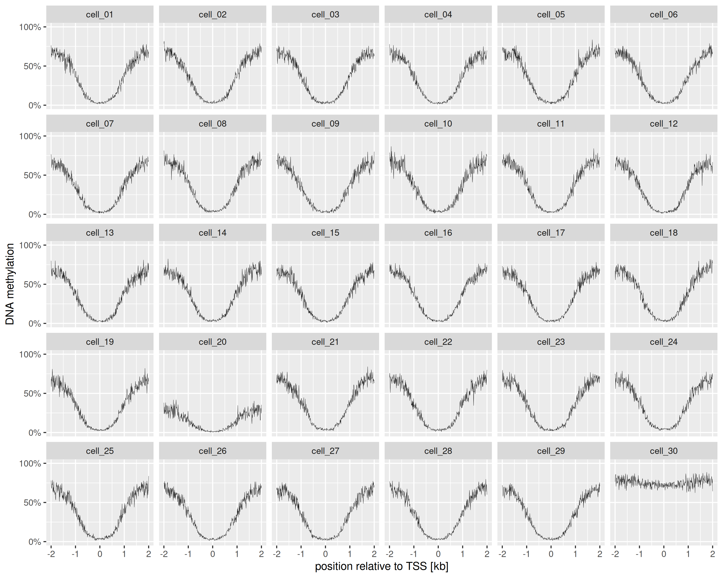
TSS profiles
Total runtime, from getting the BED files and regions to making the query, calculating the summaries and plotting: 2.489s elapsed (5.307s cpu). With methscan, generating the TSS methylation profiles alone took 11 seconds.
Using summarize_regions
A similar analysis can be done using the
summarize_regions() function if you only need to see the
distribution of beta means by file, rather than means by relative
position per file
library("ggridges")
tss.means <- summarize_meth_regions(
  bedfiles,
  tss.for_query,
  aligner = "bismark",
  fun = "mean",
  mval = FALSE
) |> as.data.table()
## [11:28:24.770899] [iscream::summarize_regions] [info] Summarizing 21622 regions from 30 bedfiles
## [11:28:24.770922] [iscream::summarize_regions] [info] using mean
## [11:28:24.770925] [iscream::summarize_regions] [info] with columns 4, 5 as coverage, beta
ggplot(tss.means, aes(x = beta.mean, y = file, fill = after_stat(x))) +
  geom_density_ridges_gradient() +
  scale_fill_distiller(palette = "BrBG") +
  theme_classic()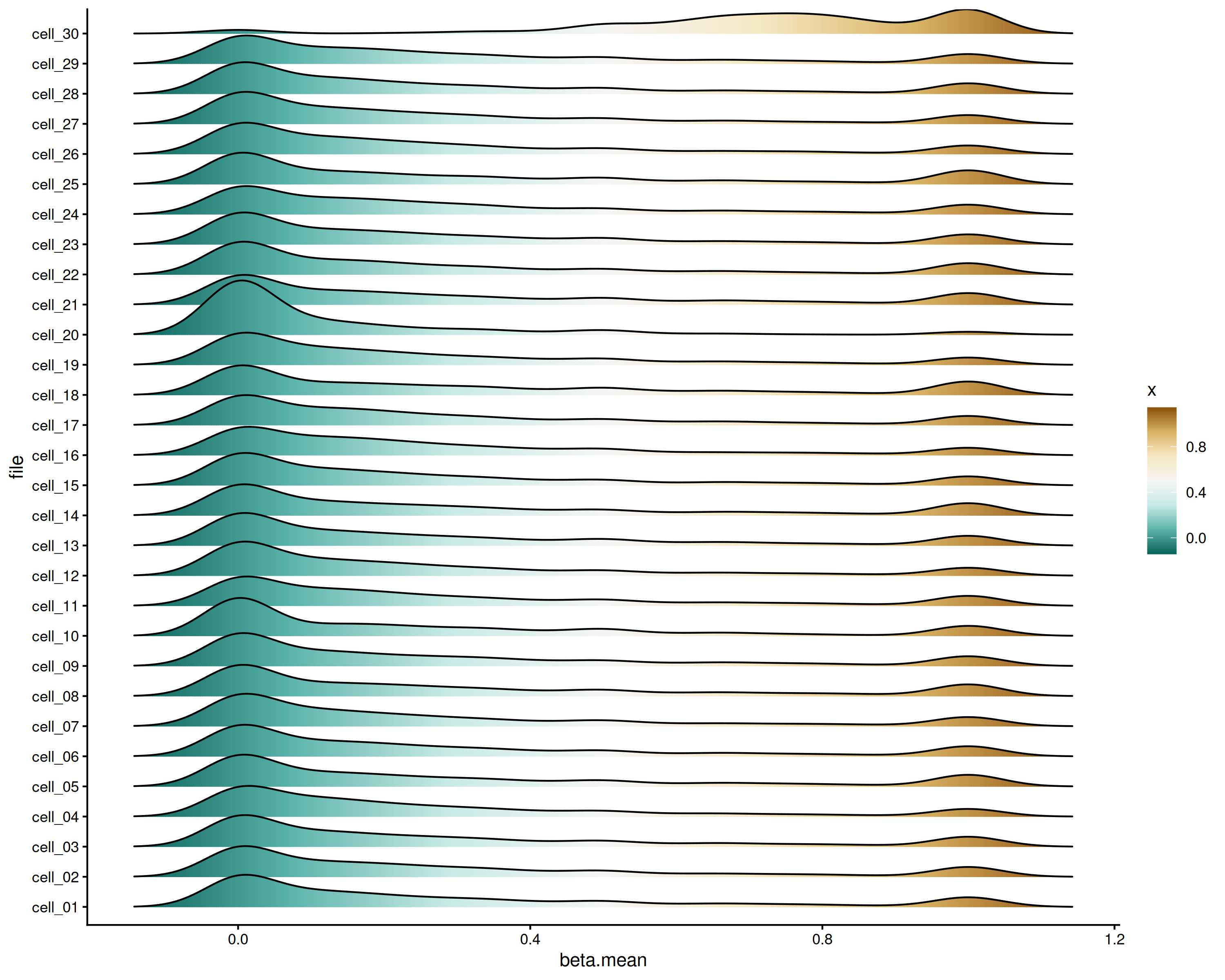
TSS distribution by file
For per-file means you could collapse the means within file:
tss.means[, .(beta.mean = mean(beta.mean, na.rm = TRUE)), by = file] |>
  ggplot(
    aes(
      x = reorder(file, beta.mean),
      y = beta.mean)
    ) +
  geom_bar(stat = 'identity') +
  theme_classic() +
  coord_flip() +
  labs(x = "Sample")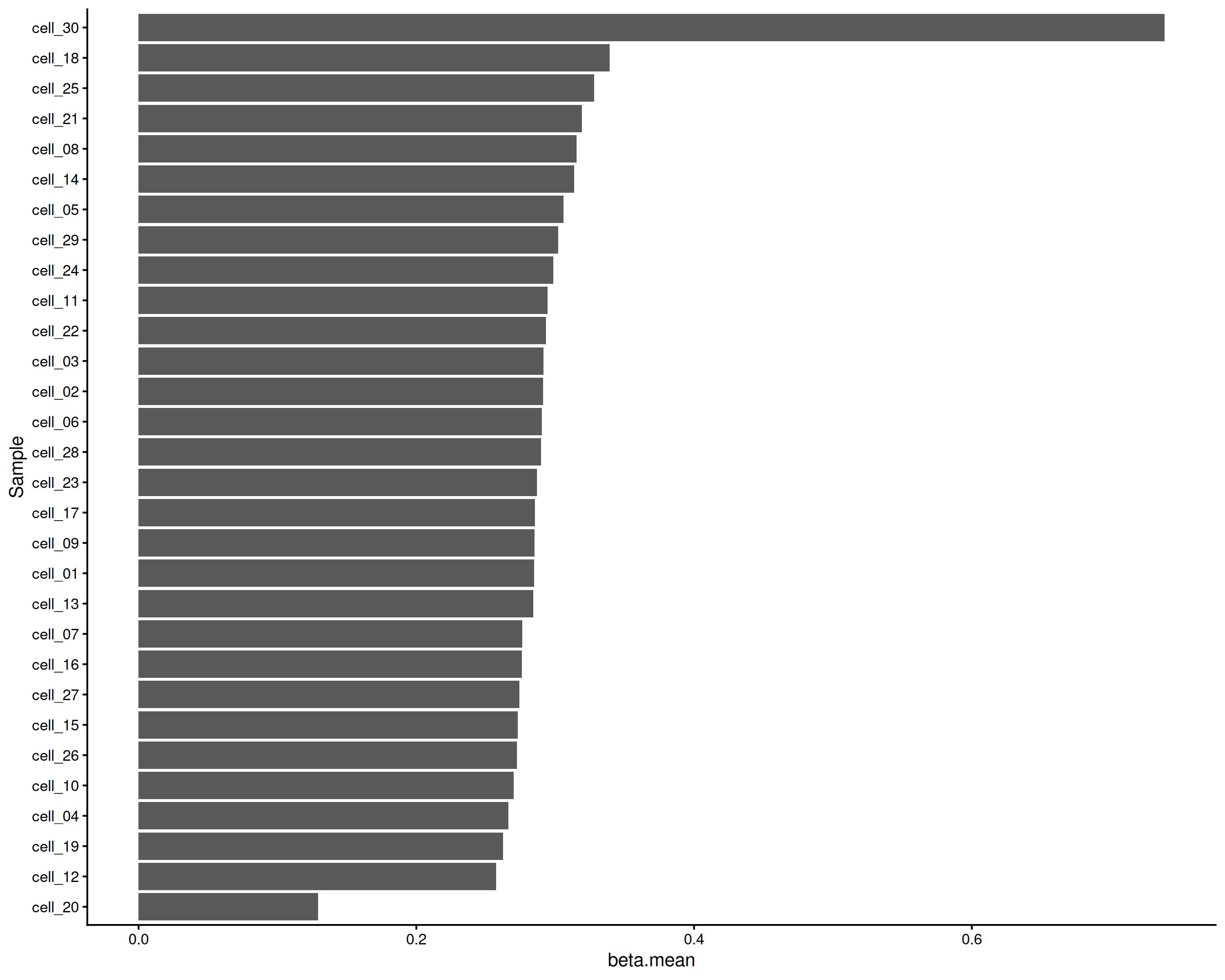
Mean TSS by file
Session info
## R version 4.5.1 (2025-06-13)
## Platform: x86_64-pc-linux-gnu
## Running under: Ubuntu 24.04.2 LTS
##
## Matrix products: default
## BLAS/LAPACK: /nix/store/yf6dpab0gcjr9gvpww1zlafs9n0f48h3-blas-3/lib/libblas.so.3;  LAPACK version 3.12.0
##
## locale:
##  [1] LC_CTYPE=en_US.UTF-8       LC_NUMERIC=C
##  [3] LC_TIME=en_US.UTF-8        LC_COLLATE=en_US.UTF-8
##  [5] LC_MONETARY=en_US.UTF-8    LC_MESSAGES=en_US.UTF-8
##  [7] LC_PAPER=en_US.UTF-8       LC_NAME=C
##  [9] LC_ADDRESS=C               LC_TELEPHONE=C
## [11] LC_MEASUREMENT=en_US.UTF-8 LC_IDENTIFICATION=C
##
## time zone: America/Detroit
## tzcode source: system (glibc)
##
## attached base packages:
## [1] stats     graphics  grDevices utils     datasets  methods   base
##
## other attached packages:
## [1] ggridges_0.5.7       BiocFileCache_2.99.6 dbplyr_2.5.1
## [4] ggplot2_4.0.0        data.table_1.17.8    iscream_0.99.9
##
## loaded via a namespace (and not attached):
##  [1] Matrix_1.7-4          bit_4.6.0             gtable_0.3.6
##  [4] dplyr_1.1.4           compiler_4.5.1        filelock_1.0.3
##  [7] tidyselect_1.2.1      Rcpp_1.1.0            blob_1.2.4
## [10] parallel_4.5.1        scales_1.4.0          fastmap_1.2.0
## [13] lattice_0.22-7        R6_2.6.1              labeling_0.4.3
## [16] generics_0.1.4        curl_7.0.0            httr2_1.2.1
## [19] knitr_1.50            tibble_3.3.0          stringfish_0.17.0
## [22] DBI_1.2.3             pillar_1.11.1         RColorBrewer_1.1-3
## [25] rlang_1.1.6           cachem_1.1.0          xfun_0.53
## [28] S7_0.2.0              bit64_4.6.0-1         RcppParallel_5.1.11-1
## [31] memoise_2.0.1         RSQLite_2.4.3         cli_3.6.5
## [34] withr_3.0.2           magrittr_2.0.4        grid_4.5.1
## [37] pbapply_1.7-4         rappdirs_0.3.3        lifecycle_1.0.4
## [40] vctrs_0.6.5           evaluate_1.0.5        glue_1.8.0
## [43] farver_2.1.2          parallelly_1.45.1     purrr_1.1.0
## [46] tools_4.5.1           pkgconfig_2.0.3